Predictive Metrics, MicroStrategy and the Social Explorer

Data science and machine learning are all the rage now – but it’s funny to think that MicroStrategy has had predictive metrics for as long, if not longer, than the 10 years I have been at the company.

Looking back at all the projects I have worked on, I am pretty certain that we never got round to using predictive metrics in anything other than an interesting exercise when project pressures permitted.

I would put this down to the early (or lack of) maturity of the data and analytical ecosystem, where getting the fundamentals right – to understand what happened in the past – was enough of an achievement without complicating the issue by trying to look forward. Another factor was the relative complexity involved in deploying predictive metrics until R integration came in to play.

Now, with a good mix of data knowledge and software capability, it is becoming possible to consider machine learning and data science as part of a analytical offering. I can see this happening at my customers, and I am also at this stage with my Social Explorer project.

The Social Explorer

I’ve been building up for a while a set of data relating to demographic and societal measures for the UK as a whole, and also down to local geographical subdivisions. Those are:

• Local Authority (LAD): Representing a local government area
• Lower-level Super Output Area (LSOA): A census area representing on average 1000 to 2000 people.
• Constituencies: A political division that returns a member of parliament

These geographical subdivisions are the backbone of my social explorer project, permitting me to join all manners of interesting data sets:

• Index of Multiple Deprivation 2015 study (by LSOA)
• Crime data by month by LSOA
• Health related data, by LSOA
• Ethnic data, by LSOA
• Migration data, by LSOA
• Referendum result, by LAD
• Election results, by Constituency

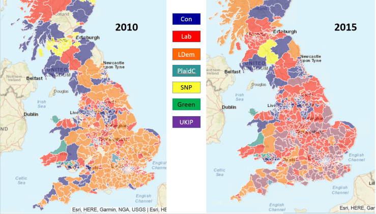
I make extensive use of maps, and have created a number of custom ones that allow me to show measures by area (LSOA, LAD, Constituency).

Putting it all together, I have a number of applications that have helped me understand the EU referendum, the 2015 election, the rise of crime in the last few years and many other useful offerings.

Has it had any value ? I think so. First, it’s been essential in helping to learn about the new features of the frequent MicroStrategy releases. Then, it’s also a useful way to find out the most efficient patterns that would help a similar application move from the exploration phase to the exploitation phase. And finally, it’s permitted me to verify, and sometimes anticipate,  current affairs stories where data or statistics play an important part.

Predictive exploration

I’ve now acquired a good knowledge of all the data I have used for this project. Throughout the discovery, I’ve often found that an endless series of questions can be asked of the data once you see a pattern or an interesting anomaly develop.

For the purpose of this article, and my initial foray into this field, I am asking two questions:

1. Is it possible to classify all the LSOAs within a LAD to gain an idea of the quality of life in each LSOA ?
2. Is it possible to predict an LSOA’s propensity for high crime deprivation based on other measures ?

Spoiler alert: I’ve not yet reached the point where I can answer these questions with absolute certainty. This is an exploration, and whilst the technology is definitely there, a fully successful approach to the problem requires iteration and experience…

Looking at the available documentation, and equipped with the R integration pack (installed seamlessly as part of the 10.11 upgrade, thank you MicroStrategy), I decided to tackle each question thus:

1. The quality of life question will be explored by the use of the k-means R function.
2. The propensity for crime will be explored by using a Naive Bayes R function.

The seasoned data scientists amongst you might scoff at my choice – the documentation itself refers to these functions as not the absolute best for the problem. Still, this is a discovery process and you have to start somewhere.

K-Means

According to the documentation:

k-Means clustering is a popular clustering algorithm that groups items into k distinct clusters so that items within the same cluster are more similar to each other than items within different clusters.

That looks like it will do the job. Having built a data set in a Dossier, placing the LSOA code and a number of pertinent metrics, the next task is to create the predictive metric.

The screen shot below shows the metric, and the data set components.

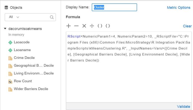
This metric calls an R function which returns a cluster value (1 to 4 in this case, you can set the metric to decide how many clusters are optimal) grouping the LSOAs according to their similarity. Below you can see a map of the area, with each LSOA shaded based on the value returned by this metric:

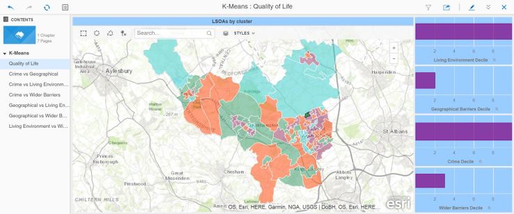
I have selected the area where I live (dark green on the map) and you can see the four metrics that I have used as parameters to the k-means function. The dossier then allows you to click on different LSOAs and verify that the clustering makes sense. You can then see that cluster values do indeed group LSOAs that have a certain profile from the combination of the four metrics.

I wanted to find out more about how the algorithm went about its classification, so I created a series of bubble charts showing for pairs of metrics the LSOA, coloured by cluster value.

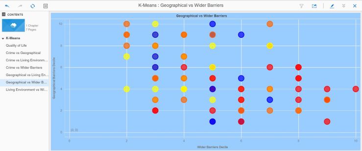
Job done, in my opinion. Or is it ? Are there other measures that can be used to better cluster these LSOAs ? I referred earlier to the iterative nature of the discovery process – given more time, I would do just that – run this for many or all of the possible metric combinations.

What can this be useful for ? Answering the quality of life question, I can now propose a classification of LSOAs according to quality of life type and ‘flavour’ (moderate crime, great living environment and so forth).

I also suspect that this might have value as a precursor step to the next challenge, the prediction of crime propensity based on certain measures.

Naive Bayes

Again, according to the documentation:

Naïve Bayes is a simple classification technique wherein the Naïve assumption that the effect of the value of each variable is independent from all other variables is made. For each independent variable, the algorithm then calculates the conditional likelihood of each potential class given the particular value for that variable and then multiplies those effects together to determine the probability for each class. The class with the highest probability is returned as the predicted class.
Even though Naïve Bayes makes a naïve assumption, it has been observed to perform well in many real-world instances. It is also one of the most efficient classification algorithms with regard to performance.

This is slightly more involved. It requires a training metric, that prepares a scoring model, and a predicting metric that uses the model to score a larger data set.

Let’s look at these metrics:

Above is the training metric. The data set is the Index of Multiple Deprivation database entries for Dacorum, the local authority where I live. I will use this dataset to train the metric. The metric HasCrime is a boolean metric that is 0 if the crime decile is 6 or above (1 is bad, 10 is good), otherwise it’s 1. This metric is used to train the model which will return its score based on the other metrics used here. When the dossier is run, the training metric will score each LSOA and write the model back to a file that the predictive metric to score a wider data set.

Below is the predictive metric. It looks very much the same, except for one value switching the training off. The metric will now use the file containing the model and score the dataset, which in this case is the full list of all LSOAs in England.

We now have a training dossier, and a predicting dossier. Below is the training dossier – I’ve added a metric that checks the correctness of the scoring.

And here’s the predicting dossier. It shows a distribution, for the selected local authority, of all the LSOAs by Crime Decile (remember, 1 is bad, 10 is good).

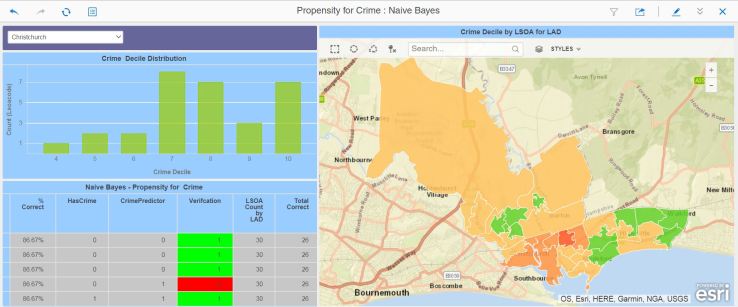
In this case, we’ve got quite a good score match – the model predicted correctly for 86% of the LSOAs. However:

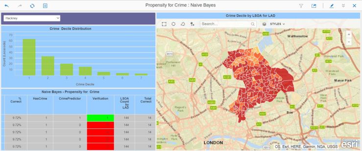
For this local authority, the model got it completely wrong ! Cycling through the local authorities, I noticed that the scoring success was variable, ranging from appalling to very good, and there appeared to be a relationship between the decile distribution and the scoring accuracy.

Conclusion

I have been able to create these predictive metrics and their accompanying dossiers quickly and without difficulty. As a result I  have managed to provide an answer to both my questions. I am unsure whether the answers are correct, though. The k-means method appeared to cluster the LSOAs in an understandable way.

The Naive Bayes method requires more work – the number of misses would make it extremely dangerous if used in an AI/Machine learning scenario. It’s possible that you need to cluster all the LSOAs, and then train and score each cluster individually to improve accuracy. It’s highly possible that the wrong scoring metrics have been used, as well.

So it’s a partial success – far more permutations of clustering and scoring metrics need to be tried to increase the accuracy of the model. Still, early days…